In many machine learning implementations, one common thing you'll notice is PyTorch.

We often skim through the code without fully understanding what each part is doing.

In this article, we'll start changing that by building a neural network from scratch using PyTorch.

Along the way, we'll explore how to:

• Define weights and biases
• Perform forward propagation
• Make predictions from input data
• Learn from training examples using backpropagation
• Update parameters using gradient descent

Before we begin building the network, let's first familiarize ourselves with the core PyTorch modules we'll be using.

Importing PyTorch

The torch module is the foundation of PyTorch.

import torch

We'll use it to create tensors, which are the data structures that store all the numerical values used by a neural network, including:

• input data
• weights
• biases

Next, we'll import the torch.nn module.

import torch.nn as nn

This module provides the building blocks for creating neural networks. It includes classes that let us define layers, parameters, and neural network models.

We'll also import torch.nn.functional.

import torch.nn.functional as F

This module contains many useful functions used in neural networks, including activation functions such as ReLU, which we'll use later when implementing our network's forward pass.

Finally, we'll import the optimizer we'll use to train our model.

from torch.optim import SGD

SGD, short for Stochastic Gradient Descent, is an optimization algorithm. During training, it updates the model's parameters so that the neural network gradually makes better predictions.

Now that we have everything imported, we can start building our first neural network.

Creating a Neural Network

Now that we have imported the modules we'll need, let's start building our neural network.

In PyTorch, neural networks are typically defined by creating a Python class that inherits from nn.Module.

class MyBasicNN(nn.Module):

Here, we've created a class called MyBasicNN.

By inheriting from nn.Module, our class gains all the functionality needed to behave like a PyTorch neural network. This includes the ability to store trainable parameters, perform forward passes, and work seamlessly with PyTorch's optimization and automatic differentiation features.

Next, we need to define how our neural network is initialized.

class MyBasicNN(nn.Module):
    def __init__(self):
        super().__init__()

The __init__() method is the constructor for our neural network. It is called automatically whenever we create a new instance of MyBasicNN.

Inside the constructor, we call:

super().__init__()

This initializes the parent nn.Module class and sets up all the internal functionality that PyTorch needs to manage our neural network correctly.

At the moment, our neural network doesn't actually contain anything. Next, we'll begin adding its weights and biases.

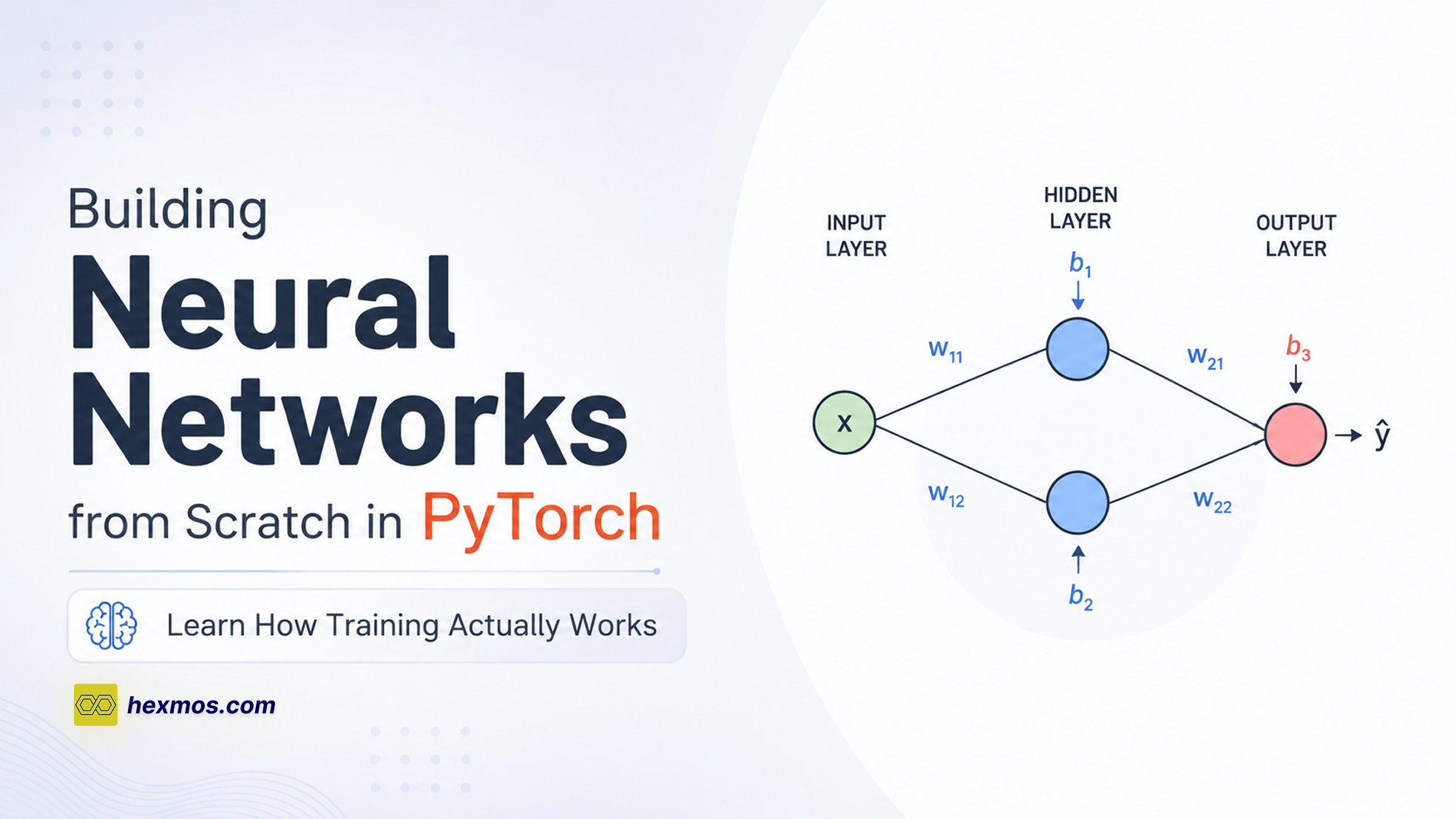
Choosing an Example Problem

Before we start adding weights and biases to our neural network, we first need an example problem to work with.

Throughout this guide, we'll recreate the following neural network using PyTorch.

This is a small feedforward neural network with:

• one input
• two hidden neurons that use the ReLU activation function
• one output neuron

The diagram also shows the values of every weight and bias in the network.

Rather than starting with random values, we'll hardcode these values into our model. This allows us to focus on understanding how a neural network is represented in PyTorch before we move on to training it.

Once we've recreated this network, we'll run inputs through it, verify that it produces the expected outputs, and then later learn how PyTorch can automatically optimize its parameters using gradient descent.

Let's begin by adding the weights and biases shown in the diagram to our neural network.

Initializing Weights and Biases

Now that we've chosen the neural network we'll recreate, the next step is to add its weights and biases to our model.

We'll start with the neural network class we created earlier.

class MyBasicNN(nn.Module):
    def __init__(self):
        super().__init__()

Let's begin by adding the first weight. From the diagram, its value is 1.70.

class MyBasicNN(nn.Module):
    def __init__(self):
        super().__init__()

        self.w00 = nn.Parameter(
            torch.tensor(1.7),
            requires_grad=False
        )

Here, we've created a variable named w00 and defined it as an nn.Parameter.

An nn.Parameter is a special type of tensor that PyTorch recognizes as belonging to the neural network. By storing weights and biases as parameters, PyTorch can automatically keep track of them and optimize them during training.

The value is wrapped in torch.tensor() because PyTorch performs all of its computations using tensors.

Notice that we've also set:

requires_grad=False

The requires_grad argument tells PyTorch whether this parameter should be updated during training.

Since we're recreating a neural network with known weights and biases, we don't want this value to change, so we set it to False.

We can initialize the remaining weights and biases in exactly the same way.

class MyBasicNN(nn.Module):
    def __init__(self):
        super().__init__()

        self.w00 = nn.Parameter(torch.tensor(1.7), requires_grad=False)
        self.b00 = nn.Parameter(torch.tensor(-0.85), requires_grad=False)
        self.w01 = nn.Parameter(torch.tensor(-40.8), requires_grad=False)

        self.w10 = nn.Parameter(torch.tensor(12.6), requires_grad=False)
        self.b10 = nn.Parameter(torch.tensor(0.0), requires_grad=False)
        self.w11 = nn.Parameter(torch.tensor(2.7), requires_grad=False)

        self.final_bias = nn.Parameter(torch.tensor(-16.0), requires_grad=False)

At this point, our neural network contains all of the weights and biases shown in the diagram.

The next step is to define how these values are used to transform an input into an output. We'll do that by implementing the network's forward() method.

Writing the Forward Pass

Now that our neural network contains all of its weights and biases, the next step is to define how an input moves through the network.

In PyTorch, this is done by implementing a method called forward(). Whenever we pass data into our model, PyTorch automatically calls this method to compute the output.

Here's the complete implementation:

def forward(self, input):
    input_to_top_relu = input * self.w00 + self.b00
    top_relu_output = F.relu(input_to_top_relu)
    scaled_top_relu_output = top_relu_output * self.w01

    input_to_bottom_relu = input * self.w10 + self.b10
    bottom_relu_output = F.relu(input_to_bottom_relu)
    scaled_bottom_relu_output = bottom_relu_output * self.w11

    input_to_final_relu = (
        scaled_top_relu_output
        + scaled_bottom_relu_output
        + self.final_bias
    )

    output = F.relu(input_to_final_relu)
    return output

Let's walk through what each part of this method is doing.

Computing the Top Branch

Here, the top branch refers to the sequence of steps labeled 1 to 4 in the diagram below.

The first calculation computes the input to the top ReLU neuron.

input_to_top_relu = input * self.w00 + self.b00

Here, we multiply the input by the weight w00 and then add the bias b00.

Next, we pass the result through the ReLU activation function.

top_relu_output = F.relu(input_to_top_relu)

Finally, we multiply the activated value (marked as 1 in the diagram) by another weight (marked as 2 in the diagram).

scaled_top_relu_output = top_relu_output * self.w01

At this point, we've completed all the computations for the top branch of the network.

Computing the Bottom Branch

The bottom branch performs exactly the same sequence of operations using a different set of weights and biases. (Marked as 1 to 5 in the diagram below)

input_to_bottom_relu = input * self.w10 + self.b10
bottom_relu_output = F.relu(input_to_bottom_relu)
scaled_bottom_relu_output = bottom_relu_output * self.w11

Just like before, we:

1. multiply the input by a weight,
2. add a bias,
3. apply the ReLU activation function,
4. scale the output using another weight.

Combining Both Branches

Finally, we combine the outputs from both branches (marked as 1 and 2 in the below diagram) and add the final bias (Marked as 3 in the diagram).

input_to_final_relu = (
    scaled_top_relu_output
    + scaled_bottom_relu_output
    + self.final_bias
)

This value is then passed through one final ReLU activation function to produce the network's prediction.

output = F.relu(input_to_final_relu)
return output

With the forward() method complete, our neural network is now fully defined. It knows how to transform an input into an output using the weights, biases, and activation functions we've provided.

The next step is to test our model by passing some input values through it and examining the predictions it produces.

Testing the Model

Now that we've finished building our neural network, let's test it to make sure it behaves as expected.

To do that, we'll generate a range of input values, pass them through the model, and visualize the predictions.

Creating the Input Values

We'll begin by generating a sequence of values between 0 and 1.

input_doses = torch.linspace(start=0, end=1, steps=11)

The torch.linspace() function creates a tensor containing evenly spaced values over a specified interval.

In this example, it generates 11 values between 0 and 1, including both endpoints.

Printing the tensor produces:

tensor([
    0.0000, 0.1000, 0.2000, 0.3000, 0.4000,
    0.5000, 0.6000, 0.7000, 0.8000, 0.9000,
    1.0000
])

These values will be used as inputs to our neural network.

Creating the Model

Next, we create an instance of our neural network.

model = MyBasicNN()

This gives us a model that contains the weights, biases, and forward() method we implemented earlier.

Running the Forward Pass

Now we can pass all of the input values through the model.

output_values = model(input_doses)

Notice that we never call forward() directly.

Instead, we simply call the model like a function:

model(input_doses)

PyTorch automatically invokes the forward() method behind the scenes and returns the predicted outputs.

Visualizing the Predictions

Finally, let's plot the model's predictions.

import seaborn as sns
import matplotlib.pyplot as plt

sns.set(style="whitegrid")

sns.lineplot(
    x=input_doses,
    y=output_values,
    color="green",
    linewidth=2.5
)

plt.xlabel("Dose")
plt.ylabel("Effectiveness")

Running this code produces the following graph.

The graph shows how the neural network's predicted effectiveness changes as the input dose increases. Since we initialized the model with known weights and biases, these predictions match the behavior of the neural network shown in our original diagram.

At this point, we've successfully built a neural network from scratch and verified that it produces the expected outputs.

So far, every weight and bias in our model has been fixed. In the next section, we'll make one of those parameters trainable and use gradient descent to learn its value from data.

Making Neural Network Trainable

So far, the network is fully hardcoded. All weights and biases are fixed constants, which means the model can produce outputs but it cannot learn from mistakes.

To enable learning, we create a trainable version of the network. This is where we switch from a static computation graph to something that can be optimized using backpropagation in PyTorch.

We define a new model called MyBasicNN_train.

Creating a Trainable Model

We copy the original network structure, but change one key thing: we allow only specific parameters to be updated during training.

class MyBasicNN_train(nn.Module):
    def __init__(self):
        super().__init__()

        self.w00 = nn.Parameter(torch.tensor(1.7), requires_grad=False)
        self.b00 = nn.Parameter(torch.tensor(-0.85), requires_grad=False)
        self.w01 = nn.Parameter(torch.tensor(-40.8), requires_grad=False)

        self.w10 = nn.Parameter(torch.tensor(12.6), requires_grad=False)
        self.b10 = nn.Parameter(torch.tensor(0.0), requires_grad=False)
        self.w11 = nn.Parameter(torch.tensor(2.7), requires_grad=False)

        self.final_bias = nn.Parameter(
            torch.tensor(0.0),
            requires_grad=True
        )

Why Only One Parameter Is Trainable

Most parameters here are intentionally frozen using:

requires_grad=False

This means they will not change during training. The idea is that we assume these internal weights are already correct, and we only want to adjust the final output shift.

The only trainable parameter is:

self.final_bias

Setting:

requires_grad=True

tells PyTorch to track this value during computation and update it during backpropagation.

In simple terms, this is the only knob the optimizer is allowed to turn.

Visualizing the Untrained Model

We can now instantiate the model and see how it behaves before training:

model = MyBasicNN_train()

output_values = model(input_doses)

sns.set(style="whitegrid")

sns.lineplot(
    x=input_doses,
    y=output_values.detach(),
    color="green",
    linewidth=2.5
)

plt.ylabel("Effectiveness")
plt.xlabel("Dose")

The key detail here is:

output_values.detach()

This removes the tensor from PyTorch’s computation graph so it can be safely plotted without tracking gradients.

Why Training Is Necessary

When we ran the model, this is the output graph that we got.

The model is clearly incorrect.

For example, at input 0.5, the output is far from the expected value of 1.0.

Instead of learning from data, the model is just producing a fixed transformation based on unoptimized parameters.

This mismatch is exactly what training fixes. The goal of backpropagation is to adjust final_bias so the output aligns with the expected labels.

Training Setup

To prepare for training, we define:

Inputs

0.0, 0.5, 1.0

Target outputs

0.0, 1.0, 0.0

These pairs form the dataset the model will learn from.

In the next step, we’ll actually make this model learn.

Preparing for Training

Creating the Optimizer

First, we create an optimizer object.

We will use Stochastic Gradient Descent (SGD) to optimize final_bias.

optimizer = SGD(model.parameters(), lr=0.1)

To optimize final_bias, we pass:

model.parameters()

to SGD.

PyTorch will automatically optimize every parameter where:

requires_grad=True

In our case, only final_bias has requires_grad=True, so that is the only parameter that will be updated during training.

Here, lr stands for learning rate, which is set to 0.1.

The learning rate controls how large each update step is during optimization.

Understanding Epochs

Before continuing, there is one important term we need to understand: epoch.

An epoch is one complete pass through the entire training dataset.

In this example, our training data contains 3 data points.

Every time all 3 training points are passed through the model once, we call it one epoch.

Running the Optimization Loop

We can now start the optimization process using a for loop that counts the number of epochs.

for epoch in range(100):
    ...

This loop will run the training process 100 times.

In other words, the model will see the full training dataset 100 times.

Tracking the Loss

Next, we initialize a variable called total_loss.

This stores the loss, which is a measure of how well the model fits the training data.

To better understand total_loss, let us look at an example.

In the figure above, the unoptimized model fits the training data poorly.

The residuals (the difference between what the model predicts and what we know is true) are large.

Because the residuals are large, the loss will also be relatively large.

Now imagine the model improves and fits the training data more closely.

The residuals become smaller.

In this case, the loss becomes smaller because the model predictions are closer to the correct values.

So, during each epoch, we use total_loss to keep track of how well the model fits the training data.

Writing the Training Loop

Now we move into the actual training process.

for epoch in range(100):
    total_loss = 0

    for iteration in range(len(inputs)):
        input_i = inputs[iteration]
        label_i = labels[iteration]

        output_i = model(input_i)

        loss = (output_i - label_i) ** 2

        loss.backward()

        total_loss += float(loss)

Running Through the Training Data

We use a nested loop to go through the entire dataset.

Each iteration picks one training example and pulls out:

• the input value (dose)
• the expected output (effectiveness)

These are stored in:

input_i
label_i

This is what the model learns from.

Getting the Predicted Output

Next, the input is passed through the model:

output_i = model(input_i)

This gives the model’s prediction for that specific input.

Calculating the Loss

Now we compare the prediction with the actual label.

We use squared error as the loss:

loss = (output_i - label_i) ** 2

If prediction matches the label exactly, the loss becomes zero.

For example:

(0 - 0)^2 = 0

That means the model got it right.

Calculating Derivatives with Backpropagation

Once the loss is computed, we trigger backpropagation:

loss.backward()

This tells PyTorch to compute how each parameter affects the loss.

In this case, it figures out how final_bias should move to reduce the error.

Tracking the Total Loss

We accumulate loss across all training examples:

total_loss += float(loss)

This gives a single number representing how bad the model is on the whole dataset for that epoch.

At this point, we have only processed the full dataset once.

Processing the Second Training Point

Now we move to the next input in the dataset.

We again take the input and label, pass it through the model, and compute the squared error.

This time, something important happens during backpropagation.

When we call:

loss.backward()

it does not overwrite previous gradients.

Instead, it adds to them.

So:

• gradients from the first point stay
• gradients from the second point are added on top

Processing the Third and Final Input

We repeat the same steps for the last training example.

Again, we compute the squared error and call:

loss.backward()

Now PyTorch adds this final contribution to the accumulated gradients from the previous two points.

After this, one full pass through the dataset (one epoch) is complete.

Checking Whether Training Should Stop

After finishing all data points, we check if the model is good enough:

for epoch in range(100):
    total_loss = 0

    for iteration in range(len(inputs)):
        input_i = inputs[iteration]
        label_i = labels[iteration]

        output_i = model(input_i)

        loss = (output_i - label_i) ** 2

        loss.backward()

        total_loss += float(loss)

    if total_loss < 0.0001:
        print("Num steps: " + str(epoch))
        break

If the total loss becomes very small, training stops early.

Otherwise, it continues for more epochs.

Taking a Step Toward a Better Bias

If the model is still not accurate enough, we update the parameter:

optimizer.step()

This uses the accumulated gradients to adjust final_bias in the correct direction.

Clearing Old Derivatives

Before the next epoch starts, we reset gradients:

optimizer.zero_grad()

Without this step, gradients from previous epochs would keep stacking up and corrupt the updates.

Tracking the Final Bias

At the end of each epoch, we print progress:

• current epoch
• current value of final_bias

This helps us see how training is improving the model step by step.

Printing the Final Optimized Bias

After training finishes, we output the final learned value:

print(
    "Final bias, after optimization: "
    + str(model.final_bias.data)
)

Watching Gradient Descent Learn

Now that the full training loop is in place, we finally get to see what all of this actually does in practice.

Before Optimization

At the start, the model is completely untrained.

The value of final_bias begins as:

0.0

This is just the default initialization, nothing learned yet.

Watching Gradient Descent Update the Bias

As the training loop runs, final_bias starts changing step by step.

Each epoch follows the same pattern:

1. Compute predictions
2. Calculate loss
3. Backpropagation computes gradients
4. Optimizer updates final_bias

And this keeps repeating.

What matters here is not a single update, but the gradual shift over many small updates. That is literally what gradient descent is doing, nudging the parameter in the direction that reduces error.

Over time, you can actually see final_bias drifting toward a better value instead of staying fixed.

After Optimization

After about 34 steps, the loss becomes very small, so training stops.

At this point, the learned value of final_bias is:

-16.0019

This is no longer random. It is the value that best fits the training data based on the loss function we defined.

Verifying the Result

To confirm that learning actually happened, we plot the updated model again:

Now the curve fits the training data much better.

The predictions align closely with the expected outputs, which shows that gradient descent did its job properly.

If you want to try the code yourself, here’s a Colab notebook you can run and experiment with

Conclusion

By the end of this article, we have seen how to create a neural network with known values, define an unknown parameter, train the model, and obtain an accurate value for that unknown while improving the model’s performance.

What we have covered here is a basic version of training. From here, you can explore more advanced use cases of PyTorch and combine it with tools like PyTorch Lightning for things like hardware acceleration and better training workflows.