Searching Billions in Seconds: How HNSW Solved the Scale Problem

We have a massive problem with how computers find things. If you have a few hundred photos on your phone, you can find one instantly, but trying to find one specific item out of a billion creates a massive technical strain.

Most systems rely on "Linear Search", which is like looking through every single page of a ten-million-page book to find one word.

This "one-by-one" approach makes real-time tools like chatbots or movie recommendations grind to a halt as the data grows. Furthermore, modern data like images or text is "high-dimensional," which breaks traditional filing systems and makes them no faster than checking every item manually.

To fix this, researchers Yu. A. Malkov and D. A. Yashunin changed the rules of the game. They realized that we don't always need a "perfect" match if it takes an hour to find; we often just need a "good enough" match found in a millisecond.

In this article, we are diving into their research paper: "Efficient and robust approximate nearest neighbor search using Hierarchical Navigable Small World graphs."

We will explore how they used a multi-layered "highway system" to make searching a billion items feel as fast as searching a hundred.

Two Methods for Fast Searching

To solve the slowness problem, the researchers combined two concepts from computer science. The first is the "Small World" phenomenon.

You’ve likely heard of "six degrees of separation", the idea that you are connected to anyone on Earth through a short chain of acquaintances.

HNSW treats data the same way. It builds a map where every data point is a "node," and similar points are connected like friends. By jumping from "friend to friend" toward your target, you can navigate a massive dataset in just a few steps.

The second concept is Hierachy, which is inspired by a structure called a Skip List.

Imagine a high-rise building where the elevators only stop at every 10th floor. To get to floor 42, you take the express elevator to floor 40 and then walk down to 42. HNSW creates "express layers" at the top with only a few data points and long-range connections.

These top layers allow the search to "skip" across the entire database to the right neighborhood instantly, before dropping down to the ground floor to find the exact result.

The Multi-Layer Highway System

To bridge the gap between speed and accuracy, the researchers introduced a multi-layer structure called a Hierarchical Navigable Small World (HNSW) graph.

You can think of this as a "highway system" for data. Instead of one giant, flat network where everything is connected, HNSW organizes data into layers.

Top Layers (Express Lanes)

These layers contain only a few data points with long-distance connections. Much like an express highway between major cities, they allow the search to "skip" across the entire dataset to reach the right neighborhood in just a few jumps.

Bottom Layers (Local Streets)

As the search moves down through the hierarchy, the layers become denser with shorter connections. Once the search reaches the ground layer—which contains every single piece of data—it uses these "local streets" to fine-tune the results and find the exact match.

This hierarchy is inspired by a data structure called a Skip List, but instead of simple linked lists, it uses complex proximity graphs.

By separating links by their "distance scales," the algorithm ensures that the search time scales logarithmically. This means that even if the dataset grows from thousands to billions, the number of steps required to find an answer stays manageable and fast.

Balancing Speed and Accuracy

To make this system work, there are a few settings that determine how the graph is built and searched.

• Connections per point (M): This is the number of "links" each piece of data creates with its neighbors. If you give each point more connections, the map becomes more detailed and accurate, but it also takes up more memory.

• The Build Effort (efConstruction): This determines how much work the system does when first creating the index. A higher setting means the "highways" and "local streets" are better connected, making future searches much more reliable.

• The Search Depth (ef): This is a setting you use during the actual search. It tells the computer how many neighbors to check before it decides it has found the best match. You can turn this up at any time to get better results without having to rebuild your entire database.

Building an HNSW Index

To see how this works, we can use a popular Python library called hnswlib. This is the same code used in the original research to prove how fast the system is. The following example shows how to set up a database and perform a search in just a few lines.

Import the Tools

We start by importing hnswlib to build the graph and numpy to handle the coordinates of our "meaning map."

import hnswlib
import numpy as np

Create the "Meaning Map"

Let's give our items coordinates based on two features: Sweetness and Size. Fruits will have high sweetness and low size, while furniture will have low sweetness and high size.

data_labels = ["Apple", "Banana", "Cherry", "Chair", "Table", "Sofa"]
data_vectors = np.array([
    [0.9, 0.2], # Apple 
    [0.8, 0.3], # Banana
    [0.9, 0.1], # Cherry
    [0.1, 0.7], # Chair
    [0.1, 0.9], # Table
    [0.2, 0.9]  # Sofa 
], dtype=np.float32)

dim = 2 # Only 2 features: Sweetness and Size
num_elements = len(data_vectors)

The data now looks like a list of coordinates. For example, Apple is at [0.9, 0.2].

Choose the Measuring Tape

We initialize the index. We use 'l2' (Euclidean distance) to measure similarity. On our map, this is just a straight line between two points; the shorter the line, the more similar the items are.

p = hnswlib.Index(space='l2', dim=dim) 

Build the Highway System

We set the rules for the HNSW structure. M sets the number of connections for each point, and ef_construction tells the system how hard to work to find the best neighbors when first building the "highways."

p.init_index(max_elements=num_elements, ef_construction=100, M=16)

Index the Data

This step takes our fruits and furniture and organizes them into layers. The "High-Sweetness" items (fruits) will naturally end up in one neighborhood, while the furniture ends up in another.

p.add_items(data_vectors)

Perform the Search

Now we search for an "Orange". We haven't told the system what an orange is, but we give it the coordinates [0.85, 0.25] (High sweetness, small size). We tell the system to find the 3 closest neighbors.

query_vector = np.array([[0.85, 0.25]], dtype=np.float32)
p.set_ef(10)
labels, distances = p.knn_query(query_vector, k=3)

The system returns the IDs for Apple, Banana, and Cherry. Even though "Orange" wasn't in our database, HNSW used the highway system to skip past the "Furniture" neighborhood and find the items that lived in the same "Sweet and Small" neighborhood.

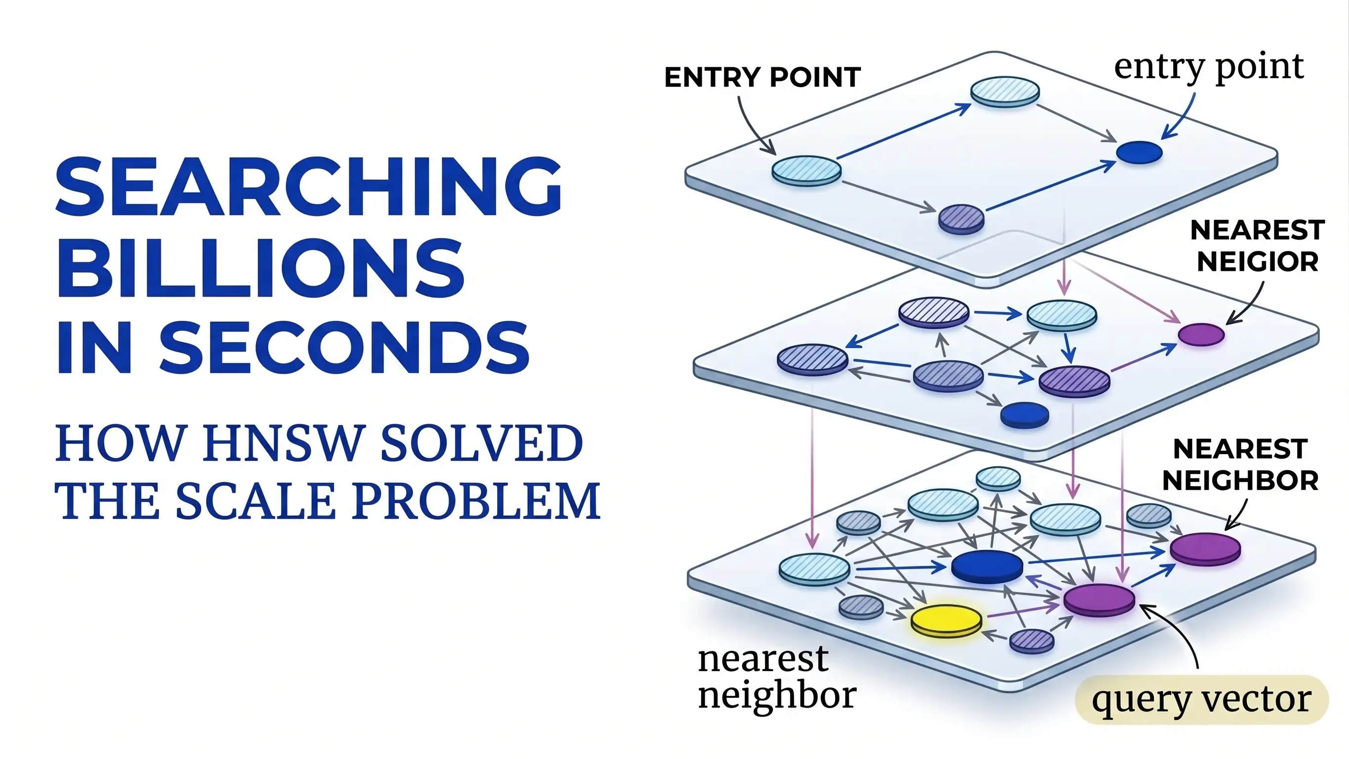
here is the layered flow diagram.

In this diagram you can see there are three layers in the graph. The top layer has only a few nodes and the bottom layer has all the nodes. The search starts from the top layer and moves down to the bottom layer.

Realworld Applications of HNSW

The reason this research paper is so influential is that it solved the "scale" problem for some of the most popular technology today. Because HNSW can find a "neighborhood" of similar ideas in milliseconds, it is used in:

AI Chatbots & RAG

When you ask an AI a question, it uses HNSW to search through millions of documents to find the specific paragraphs that contain the answer.

Recommendation Engines

Apps like Spotify or Netflix use this logic to find songs or movies that are "mathematically close" to what you just finished watching.

Image Search

Tools like Google Lens compare the "fingerprint" of your photo against billions of others to find a match instantly.

Fraud Detection

Banks use it to see if a new transaction looks "similar" to known patterns of theft or if it fits your normal "neighborhood" of spending.

Conclusion

Before this paper, we had a difficult choice: we could have a search that was perfectly accurate but incredibly slow, or a search that was fast but broke down as it grew.

Malkov and Yashunin’s HNSW changed that by introducing the "highway" system for data. By accepting a tiny bit of approximation, they gave us a way to search through billions of items in the blink of an eye.