How Netflix Uses Matrix Factorization to Predict Your Next Favorite Movie

One common issue a recommendation system faces is the lack of user interaction data. For example, on a typical OTT platform Netflix, a user might have only rated 10–20 movies. Based on such a small number of ratings, it is difficult to provide high-quality recommendations, especially when considering the millions of other movies and users in the system.

This shortage of user feedback creates a massive gap in the data known as Sparsity. Sparsity in movie recommendations can be illustrated as a giant spreadsheet where every row is a person and every column is a movie; in reality, about 99% of those cells are empty. This "emptiness" is the primary reason why building an effective recommendation engine is so challenging.

Matrix Factorization Techniques for Recommender Systems

To tackle this problem, researchers Yehuda Koren, Robert Bell, and Chris Volinsky introduced a technique called Matrix Factorization. This method directly addresses sparsity while solving other critical issues, such as:

• The Scaling Problem: As systems grow to hundreds of millions of users, it becomes computationally "expensive" and difficult to find similarities between every single person in real-time.

• Shallow Recommendations: Traditional methods often limit recommendations to simple factors like genre or actors, failing to capture the deeper, hidden reasons why we actually like a movie.

In this article, we are going to explore how this method solved these issues and improved the Netflix recommendation system, along with a step-by-step demonstration of how it works.

Latent Factors

To solve the sparsity problem, the paper moves away from movie titles and focuses on Latent Factors.

In this Latent Factor space, a trait is a hidden characteristic that describes a movie or a user’s preference. For example, one trait might be "Action Intensity," another could be "Emotional Depth," and a third might be "90s Nostalgia".

These traits aren't labeled with names like "90s Nostalgia"—they are represented simply as numbers in a list (a vector).

• movie vector(q_i) : A list of numbers representing how much of each trait the movie possesses. For a 90s action movie, the "Nostalgia" number might be high (0.9), while for a modern drama, it would be low (0.1).

• user vector(p_u) : A list of numbers representing how much of each trait the user enjoys. For a person who loves action movies, the "Action Intensity" number might be high (0.9), while for a person who dislikes dramas, it would be low (0.1).

import numpy as np

# Trait 0: 90s Nostalgia | Trait 1: Action Intensity
# Movie Vector (q_i) for a 90s Action Movie
movie_vector = np.array([0.9, 0.8]) 

# User Vector (p_u) for a user who loves 90s movies but is neutral on Action
user_vector = np.array([0.7, 0.1])

To predict how many stars a user will give a movie, the authors developed this equation:

Each part of the equation is as follows:

1. μ (Global Bias): The average rating of all movies in the system
2. b_i (Item Bias):How much better (or worse) this movie is compared to the average.
3. b_u (User Bias): How much more critical (or generous) this specific user is when giving stars.
4. q_i^T p_u (User-Movie Interaction): The dot product of the user and movie vectors, representing how much the user likes the movie based on their latent factors.

Why This Solves Sparsity

Because the system learns general traits (like "90s Nostalgia") rather than specific titles, it can predict your interest in a movie you’ve never seen. If the math learns from your history that you enjoy 90s traits, the Dot Product will automatically result in a high score for any other movie in the database that also has a high 90s trait value.

The Real Problem

Here it comes the real problem: it is impossible to manually look at millions of movies and users to find their specific trait values. To solve this, we initialize these traits by giving them random numbers at the start. These values are essentially just "noise." They don't have any real meaning yet.

self.P = np.random.normal(scale=1./self.K, size=(self.num_users, self.K))
self.Q = np.random.normal(scale=1./self.K, size=(self.num_items, self.K))

How Stochastic Gradient Descent (SGD) Discovers These Traits

Here we are going to learn how SGD helps us discover the true meaning of these traits. This is the main mathematical engine in the matrix factorization algorithm.

The SGD engine improves the model by comparing its "Guess" against the Real Rating provided by the user. Every time the machine sees how far off it is, it uses that Error to "nudge" the random numbers closer to a value that makes sense.

We can split this into three steps:

Prediction

The model uses its current (random) numbers to guess a star rating using the previous equation.

    def get_prediction(self, u, i):
        """
        Prediction = Global Average + Item Bias + User Bias + (User Vector . Item Vector)
        """
        # We add the biases and the dot product of the latent factors
        dot_product = self.P[u, :].dot(self.Q[i, :].T)
        return self.b + self.b_u[u] + self.b_i[i] + dot_product

prediction = self.get_prediction(u, i)

Error Calculation

The error is calculated by subtracting the predicted rating from the actual rating.

e = r - prediction

Update

The values of P and Q are updated based on the error.

        # We use 'alpha' to control the size of the nudge
        # and 'beta' to prevent the numbers from getting too large
        user_vec_old = self.P[u, :].copy()
        item_vec_old = self.Q[i, :].copy()
        
        self.P[u, :] += self.alpha * (e * item_vec_old - self.beta * user_vec_old)
        self.Q[i, :] += self.alpha * (e * user_vec_old - self.beta * item_vec_old)

In this equation we came through two new variables Alpha and Beta.

• Alpha - The Learning Rate: This determines how big each "nudge" is. If Alpha is too high, the system overreacts to every mistake and becomes unstable. If it is too low, the system takes forever to learn.

• Beta - The Regularization Parameter: This prevents the numbers from getting too large. This keeps the model flexible enough to predict movies the user hasn't seen yet.

Here it comes the real doubt:

How can the system predict a rating for a movie the user hasn't seen?
The system uses the ratings a user has given to build a mathematical profile of their tastes (their Latent Factors). Once the system knows what traits a user likes, it can look at any new movie, identify its traits, and calculate a predicted score.

The result

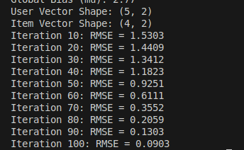
After running the Stochastic Gradient Descent (SGD) algorithm, this is the output we got. For this test, we tracked 2 latent traits for each of our 5 users and 4 movies.

The SGD algorithm successfully reduced the initial noise by "nudging" the random values over 100 iterations. By the 100th iteration, we achieved an error rate of 0.0903.

To measure this error, we used RMSE (Root Mean Square Error). It tells us, in a single number, the average distance between the stars a user actually gave and the stars our system predicted. As the RMSE value decreases our prediction accuracy increases.

Conclusion

Through this paper, we learned that Matrix Factorization effectively solves the sparsity problem by using latent factors and Stochastic Gradient Descent to discover hidden patterns in user behavior.
In the real world, this technique is used to predict individual preferences and automate personalized suggestions by mapping users and items into a shared mathematical space. Companies like Netflix and Amazon use advanced methods of this technique to recommend products to their users.