Introducing dbctx: Compile PostgreSQL Database into LLM-Friendly Context
dbctx compiles a PostgreSQL database into a compact, queryable context file. AI agents and text-to-SQL systems get only the schema, relationships, and field meaning they need, instead of the entire information_schema.

Imagine a support engineer types this question into an internal chatbot late at night:
"How many enterprise customers had a failed payment last month?"
The chatbot uses an LLM connected to your production PostgreSQL database. It writes a SQL query in seconds, runs it, and shows an answer with full confidence.
The answer is wrong.
Not because the model writes bad SQL. It guessed that "failed" means status = 'failed', when your payments table actually uses state = 'declined'. It also guessed where "enterprise" data lives, when in reality it sits three joins away, inside a JSONB field called metadata.plan.tier.
The query ran without an error and returned real rows, so no one saw a warning. Someone made a decision based on a number that was never correct.
If you have tried to build a tool like this, a text-to-SQL system, or an AI agent that answers questions about your data, you have hit this same wall. The hard part is not SQL generation; modern LLMs write SQL well. The hard part is telling the model what your database actually contains, in a way that is small enough to fit in a prompt and accurate enough to trust.
This post introduces dbctx, an open-source Go tool that solves exactly this problem. It connects to PostgreSQL, reads the real schema and the real data, and compiles all of it into one compact file called .dtx, something an AI system can query in milliseconds. Building it does not involve a generative model at all. The process is deterministic, so you build the index once and reuse it many times.
Your database is not your schema
Ask an engineering manager to describe their database and you will usually get an ER diagram. Ask an LLM to write a query against that same database, and a plain schema dump is what actually goes into the prompt:
payments(id, org_id, status, created_at, metadata JSONB)
That line is accurate, and almost useless. It lists five column names without explaining what is actually inside them.
We tested dbctx against our own production database, the one behind LiveReview, our AI code review product. It is not a small demo schema. It has:
- 60 tables
- 758 columns
- 97 foreign keys
- 558 distinct JSONB paths
We pointed dbctx at a table called reviews. A plain schema dump would never show you this, but dbctx pulls it out automatically:
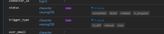
The schema declares status as character varying(50). Nothing in the schema says it can only hold four values, but it does: completed, failed, created, and in_progress. dbctx found these values by reading the actual rows.
This matters because an LLM that writes WHERE status = 'success' is not hallucinating at random. It is guessing at a value the schema never declared.
JSONB columns hide even more. A schema dump shows one line, metadata jsonb, and that single line hides 31 distinct paths in our own metadata column:
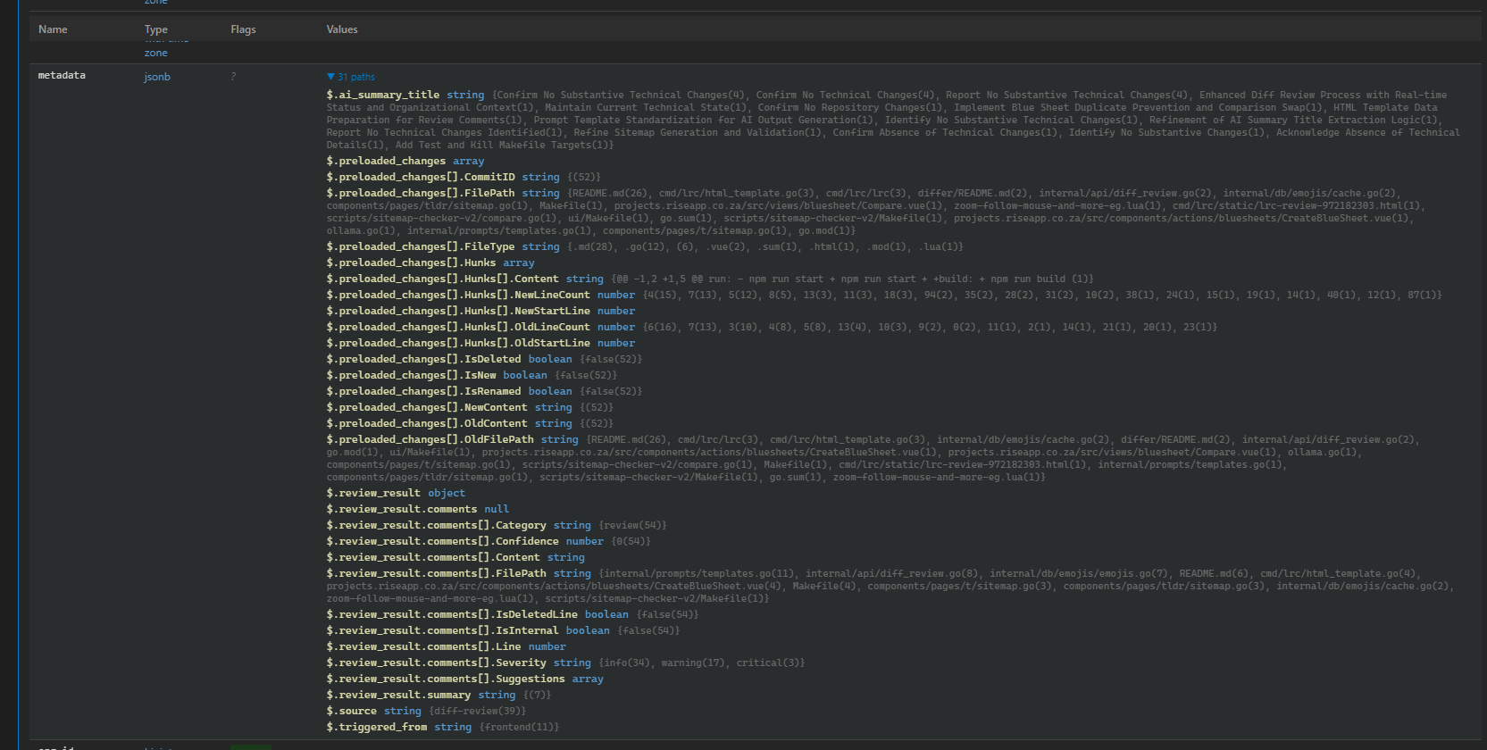
One path, $.review_result.comments[].Severity, holds the values info, warning, and critical. Another path, $.triggered_from, holds the value frontend. You cannot see any of this unless you already know to look for it, and an LLM looking at metadata jsonb has no way to know these paths exist.
A schema describes shape. It does not describe meaning. Meaning is exactly what a model needs to write a query you can trust.
Foreign keys create a related problem: they form a graph, and a flat schema dump does not walk that graph for you. A question about reviews almost always needs data from pull_requests and orgs, because that is where the joins point, and something still has to trace that path, whether it is a person or a tool.
Size is the last problem. Our own database's full schema, written as plain text, runs to several thousand tokens before the model has even seen your actual question. Now scale that up: a real enterprise system might have 500 tables and 6,000 columns, and a full dump for that system could reach tens of thousands of tokens, enough to fill most of a modern context window before your question arrives.
That is not just expensive, it actively hurts accuracy. The model has to search through hundreds of irrelevant tables to find the ten that matter, and every extra token is a chance for it to lose focus.
Compile it like source code
There is a useful comparison here, and it is also where the name dbctx comes from.
You do not ship raw .go source files to production and make the runtime parse them on every request. You compile the code once, producing a small artifact built for the runtime, and you ship that artifact instead.
dbctx treats your database the same way. It connects to PostgreSQL, reads the schema, samples the data, and maps the JSONB structure. Then it compiles all of this into one .dtx file, a portable SQLite database that is the "compiled" version of your Postgres instance.
Your live database stays the source of truth. The .dtx file is what you actually hand to an AI system. This file is:
- Small enough to version and cache
- A plain SQLite file, so any SQLite tool can open it directly
- Fast enough to query in milliseconds
- Reusable, so you never re-introspect Postgres on every request
Here is the full path from a live database to an answer:
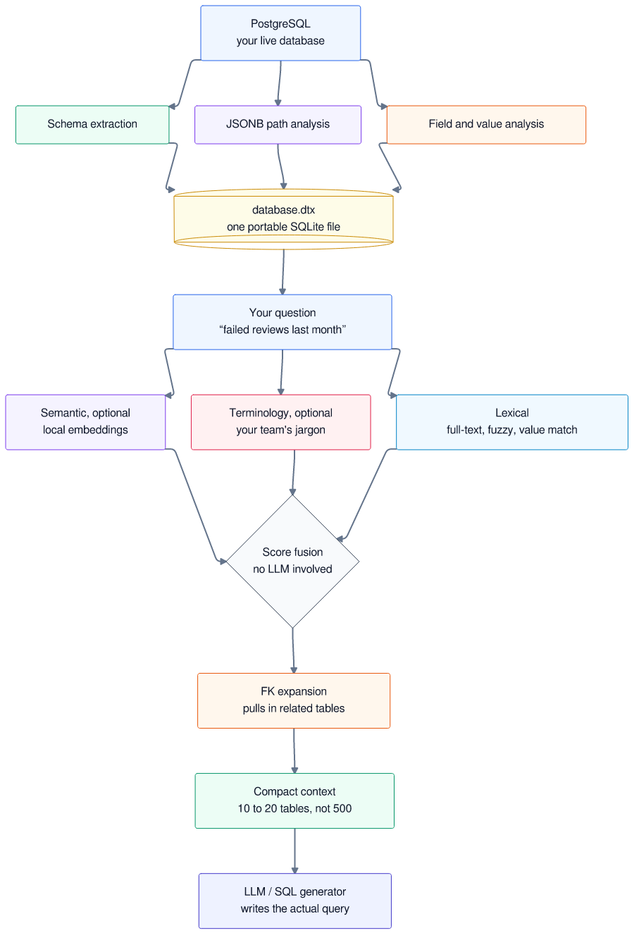
Look closely at this diagram. Every deep dive later in this post zooms into one box here.
The left half is the core index, built from deterministic introspection alone: no API key, no inference server, no generative model involved.
The right half turns a question into a ranked, joined, trimmed set of tables, and that process is deterministic too.
An LLM enters the picture in only two places:
- At the very end, where it writes the actual SQL.
- Off to the side, where it optionally helps a human build a terminology dictionary (more on this later).
What actually gets built
Running dbctx build produces three layers of understanding. Each layer builds on the one before it.
| Layer | What it captures |
|---|---|
| Structural | Tables, columns, types, primary keys, foreign keys, indexes |
| Derived | Enum-like and state-like fields, representative values and their frequencies, JSONB paths and inferred types |
| Retrieval | A full-text index, an optional local semantic index, an optional terminology dictionary, and logic to expand results through foreign keys |
The structural layer is what any introspection tool gives you. The derived layer is where dbctx does its real work: it is the difference between knowing a column exists and knowing what is actually inside it. The retrieval layer makes the whole index queryable at prompt time, instead of re-analyzed from scratch on every request.
Try it yourself:
dbctx build postgres://user:pass@localhost/mydb --output mydb.dtx
We ran this against our 60-table, 758-column production database. The full build, including schema extraction, field analysis, and JSONB analysis across every table, took about 12 seconds, roughly the time it takes to read this paragraph out loud.
The resulting file was 448 KB, smaller than most photos on your phone. You could attach it to a Slack message without a second thought.
Ask it a question
dbctx query mydb.dtx "How many failed GitHub reviews last month?"
The output is not prose. It is compact, notation-based schema, built specifically for a model to read:
--- notation ---
PK: primary key           col → table  foreign key
^  is primary key         ?  nullable   >target  FK target
[state] state-like categorical (< 100 distinct values)
[cat]   categorical field
{a, b, c}  representative values (from pg_stats)
$.path  type  {samples}  JSONB path with inferred type
(score: X.XX)  relevance score from query matching

reviews  (score: 15.24)
  PK: id
  org_id → orgs
  pull_request_id → pull_requests
  status character varying(50) [state]
    {completed, failed, created, in_progress}
  metadata jsonb
    $.provider  string  {github, gitlab}
  created_at timestamp with time zone

orgs  (score: 3.12)
  PK: id
  name text
  plan text [state]
    {free, pro, enterprise}
Two things happened here. First, reviews scored highest, because both "reviews" and "failed" matched it directly. Second, orgs appeared even though the question never mentioned it. dbctx pulled it in automatically, because reviews.org_id points to orgs, and any real query would need that join.
The legend at the top is not decoration. It tells the downstream LLM exactly how to read [state], →, and $.path, so you never have to explain this notation in your prompt.
Here is the same tool, on the same database, answering a different question:
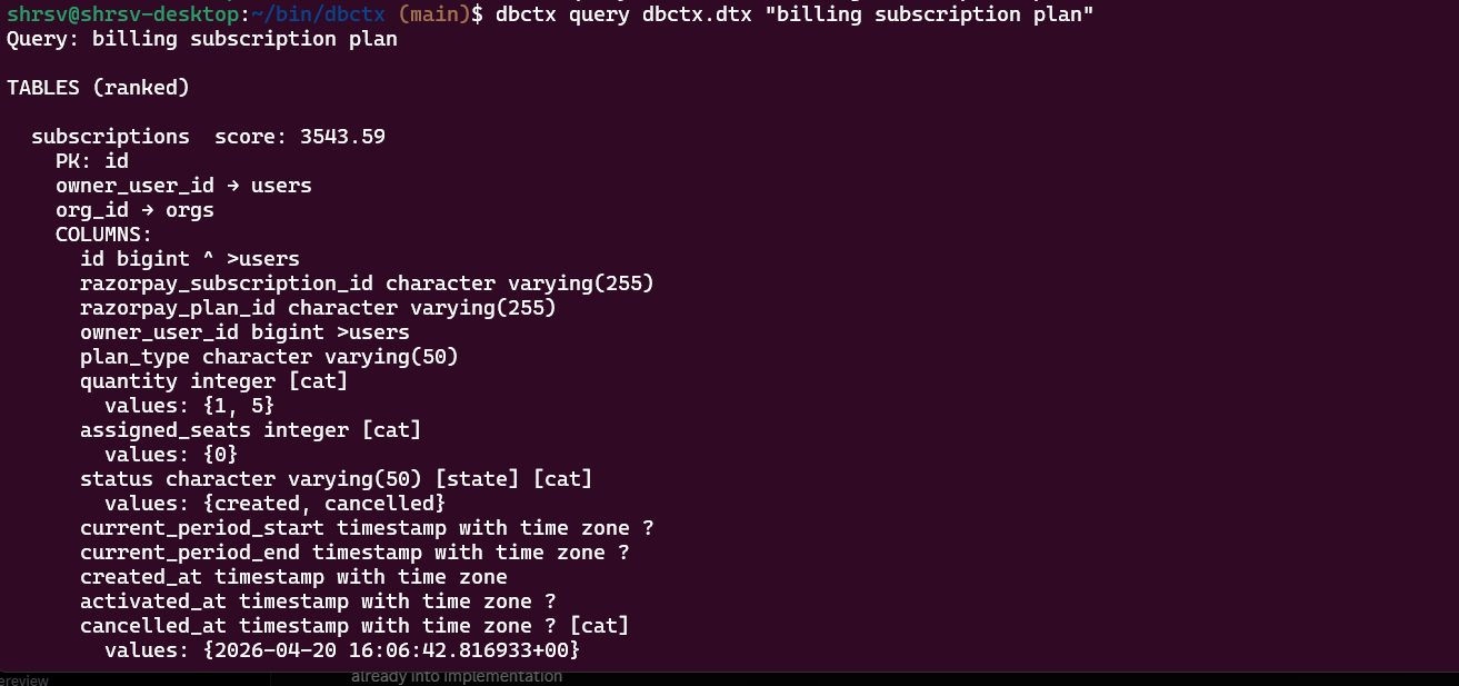
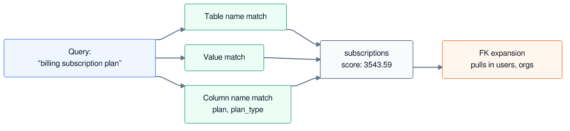
The query was "billing subscription plan". dbctx matched the subscriptions table with a score of 3543.59, pulled in its foreign keys to users and orgs, and returned that table's full column list, its state field (status, with real values created and cancelled), and its categorical fields.
That output has about 30 columns. Our full schema has 758. dbctx answered the question using under 4% of the database. The other 96% was never read by anything.
Explore the index in your browser
dbctx ui mydb.dtx
This command starts a local web explorer. It shows everything dbctx extracted, so you can check the index without writing a single query:
Overview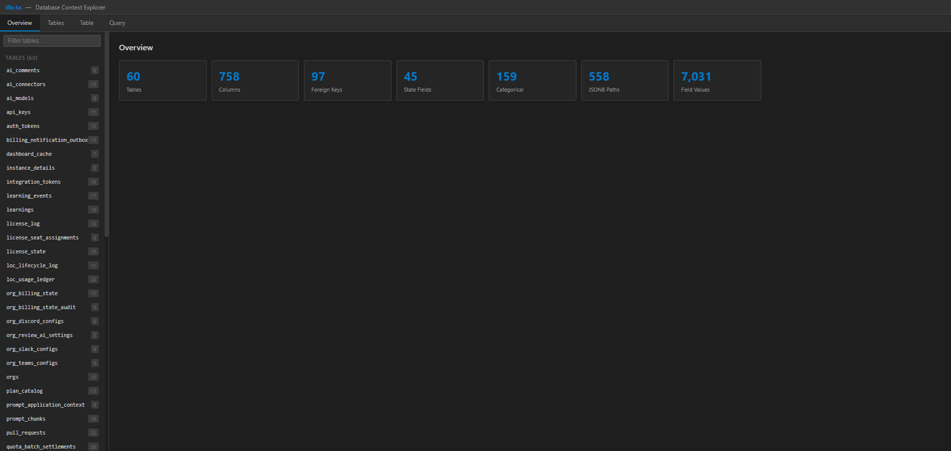 |
Table details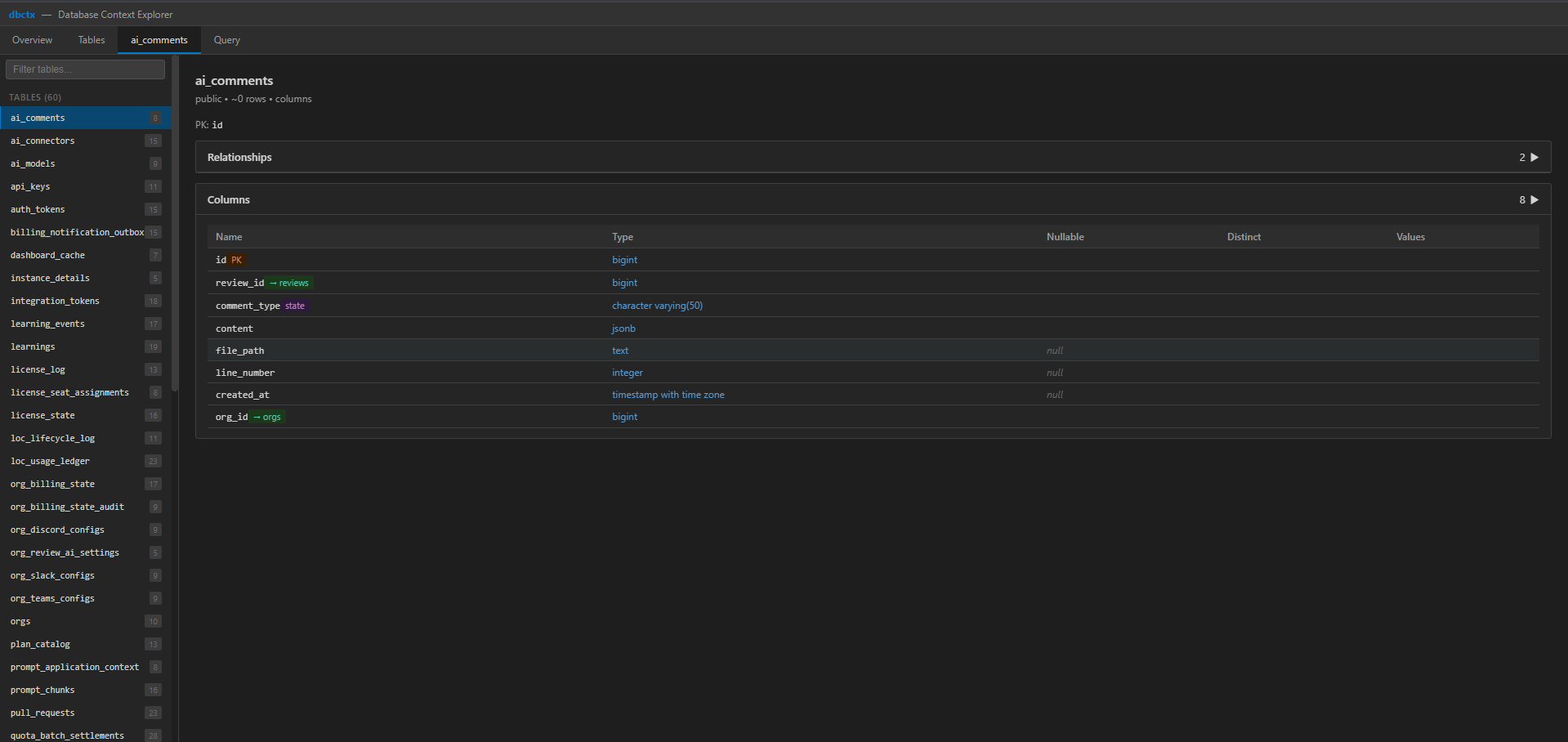 |
Query interface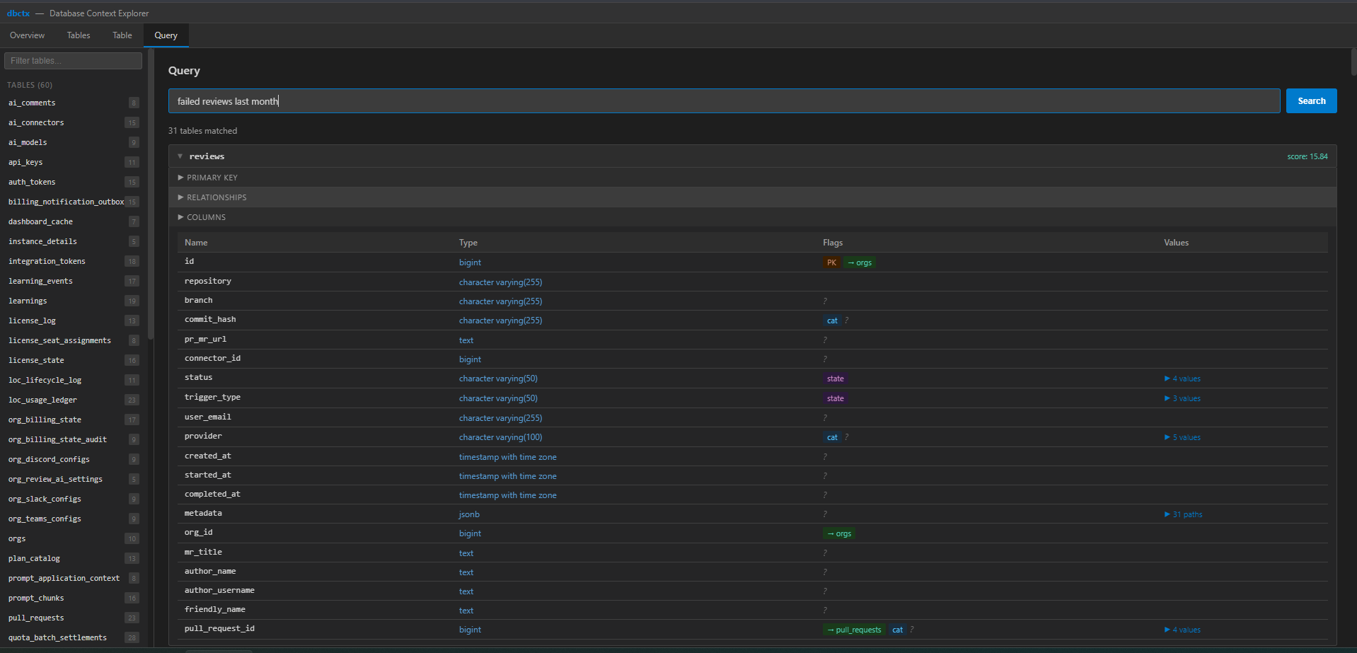 |
|
The overview panel above shows the same production database we have used throughout this post. dbctx extracted all of this automatically, with no manual documentation:
- 60 tables
- 758 columns
- 97 foreign keys
- 45 state fields
- 159 categorical fields
- 558 JSONB paths
- 7,031 distinct field values
How dbctx scores a table
Imagine two people ask dbctx different questions against the same schema: "buyers" and "customers." One question gets a perfect match. The other gets nothing. There is no table called buyers, and no amount of fuzzy matching turns "buyers" into "customers." String similarity cannot bridge that gap.
This is the real limit of lexical search, and it is exactly why dbctx does not rely on lexical matching alone.
For a direct hit, scoring works by adding up evidence: whether the query mentions a table name, a column name, a representative value stored in a column, or a JSONB path. Each match adds weight, and matches stack together.
Remember the earlier example: subscriptions scored 3543.59 for the query "billing subscription plan." The table name matched directly, the column names plan and plan_type are meaningful, and the query terms lined up with more than one signal at once.
After scoring, dbctx walks the foreign-key graph outward from every matched table. If reviews matches, orgs and pull_requests come along automatically, because a query that needs reviews almost always needs to join through them too.
For the "buyers" case, lexical scoring alone returns a wall of zeros. This is the exact reason dbctx ships an optional semantic layer.
Semantic search: finding synonyms without an API key
The semantic layer exists to catch the exact case above: a real question, phrased in words your schema does not literally contain.
It runs on a small local model, BGE-small-en-v1.5, with 384 dimensions and about 33 million parameters. For comparison, that is roughly 1,000 times smaller than the large language models people usually connect to their data. The model runs entirely on CPU. You do not need an API key, an external inference call, or a vector database.
The model file itself is about 133 MB, smaller than most mobile games. dbctx downloads it once, to ~/.dbctx, the first time you use it.
At build time, dbctx writes a short text summary for:
- Every table
- Every meaningful column (state-like, categorical, or a foreign key, not every column)
- Every notable JSONB path
dbctx embeds each summary into a vector. At query time, it embeds your question too, and compares it against these vectors with a plain cosine similarity scan. It does not use an approximate nearest-neighbor index; for one schema's worth of objects, brute force is already fast enough, and extra complexity would not help.
The important part is how dbctx combines a semantic hit with a lexical one. A naive approach would just add the two scores together, but that would let a fuzzy semantic match outrank an exact identifier hit, which is backwards. Instead, dbctx fuses the scores like this:
final_score = lexical_score + 0.6 × normalized_semantic_score × strongest_lexical_score_in_results
Here is a worked example with real numbers. Say a query lexically scores orders at 40, the strongest lexical hit in the result set. The same query semantically scores orders at 0.9 and purchases at 0.4 (normalized similarity values):
orders:40 + 0.6 × 0.9 × 40 = 61.6purchases:0 + 0.6 × 0.4 × 40 = 9.6
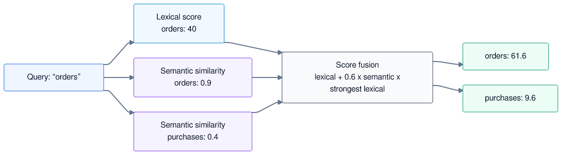
The exact identifier still wins by a wide margin, but the semantically related table now shows up in the results, instead of vanishing completely.
What if lexical search finds nothing at all? This is the "buyers" versus "customers" case. Here, the scale factor falls back to 1.0. That is not enough to let a weak semantic match dominate, but it is enough for a real match to surface, in a case where lexical search cannot help at all.
What does this cost you? At 50-table scale, around 90 embedded objects, a hybrid query runs about 43ms with the model already warm, against 7ms for lexical-only. The difference, about 36ms, is close to the time a single frame takes to render in a 24fps video. Loading the model into memory costs about 240ms, a cost you pay once per process, not once per query.
How dbctx reads JSONB columns
JSONB is the part of a schema most tools give up on. It is also often where the fields people care about most actually live: severity, plan tier, feature flags, provider metadata. dbctx does not just check the column type; it opens the documents and reads them.
Scanning every row of a large JSONB column would be wasteful, like reading an entire phone book cover to cover just to learn what a phone number looks like. So dbctx samples instead:
- Small tables, under 5,000 rows, get a plain
LIMIT 50. - Larger tables use
TABLESAMPLE BERNOULLI, at a percentage that shrinks as the table grows. A table with a million rows gets sampled at roughly 0.05%, which works out to about 500 rows actually inspected.
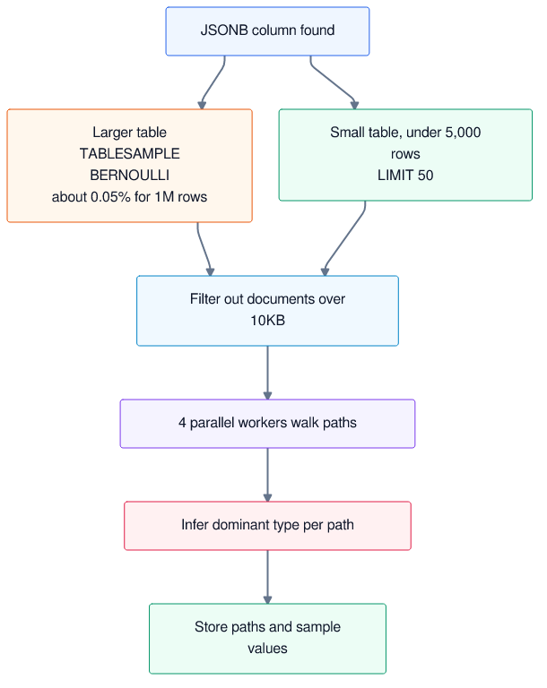
Every sample query also filters out documents over 10KB, so one huge outlier blob cannot stall the whole build. The work runs across four goroutines in parallel, and results land in a single SQLite transaction, so a build never leaves the index half-written.
For each path, dbctx must also decide what type it is. This is not always simple, because different rows can genuinely disagree. dbctx counts how often each type appears at that path across the sample, and keeps the most frequent one. For example, if $.discount is a number in 98% of rows and a string in the rest (a stray "none" value somewhere), dbctx reports it as a number.
Arrays get their own notation. $.review_result.comments[].Severity means this path exists inside every element of an array, exactly the shape you saw two sections ago, in a real screenshot of our own metadata column.
Paths with 20 or fewer distinct values get their full value list stored. This means the same {info, warning, critical} treatment that works for a flat status column also works three levels deep, inside a JSON blob.
Terminology: teaching dbctx your team's jargon
Semantic search handles "buyers" versus "customers" well, because a general-purpose model has seen both words used the same way thousands of times. But it has never seen your team's internal shorthand.
Maybe your dashboards say "LOC," but your database says lines_of_code. Or your team uses a nickname for a metric that means nothing outside your own Slack workspace. No embedding trained on public text can reliably bridge that specific gap.
So dbctx treats terminology as a third, independent signal, and it deliberately keeps an LLM out of the tool itself. You stay in control of the process:
- Generate a prompt containing your actual schema.
- Hand that prompt to whatever model you already trust, Claude, GPT, Gemini, it does not matter which.
- Work through the prompt like a conversation.
- Import the reviewed JSON back into dbctx.
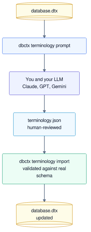
dbctx terminology prompt mydb.dtx > terminology-prompt.txt
# paste into your LLM of choice, work through it, save the JSON
dbctx terminology import mydb.dtx terminology.json
[
  {
    "term": "loc",
    "aliases": ["line of code", "lines of code", "source lines of code"],
    "targets": ["metrics.loc"]
  }
]
dbctx validates every mapping against the real schema on import. A hallucinated table name gets rejected; it is never silently trusted.
Terminology is retrieval metadata, not schema content. This means importing a thousand-entry dictionary does not add a single extra token to the context dbctx eventually hands your LLM. Terminology only changes which tables get found. It never changes how much text describes them.
A file you can check into git
Most systems treat "context for the LLM" as something assembled fresh on every request. dbctx treats the .dtx file as a build artifact instead, the same way you would treat a compiled binary or a generated OpenAPI spec.
A .dtx file is, at the end of the day, just a plain SQLite file. That is not a small detail: it means every tool that already works with SQLite, a CLI client, a GUI browser, a language driver, a diffing utility, works with a .dtx file too, directly, with no custom parser needed. You can:
- Generate it in CI
- Check it into a repo, next to
schema.sql - Inspect it with any SQLite client
- Diff two versions with a SQLite-aware tool, such as
sqldiff, since a plaingit diffwill not produce a useful diff on a binary file - Rebuild it whenever the schema changes
That last point comes with one honest caveat. A rebuild today reprocesses the whole database; there is no incremental mode yet that only re-analyzes the tables that actually changed. It is on the roadmap, but not built. In practice this has not been a problem: a full rebuild of our 758-column production database takes about 12 seconds. It is worth watching on much larger schemas, where a full rebuild will take longer.
The format is also forward-compatible. A .dtx file built before dbctx supported semantic search still opens fine on a newer version. It simply has no semantic index, and queries fall back to lexical-only, until you rebuild the file.
Performance, in numbers you can picture
Every number below comes from our own 60-table, 758-column, 97-foreign-key production database. None of it is a synthetic benchmark.
Build time
| Phase | Duration | Share |
|---|---|---|
| Connect | 0.1ms | 0.0% |
| Schema | 2.5s | 20.2% |
| Store | 11ms | 0.1% |
| Fields | 3.2s | 26.2% |
| JSONB (4 workers) | 6.5s | 53.1% |
| FTS | 49ms | 0.4% |
| Total | ~12s | 100% |
Query time
| Query | Duration | Tables matched |
|---|---|---|
"id" |
138ms | 11 |
"reviews" |
76ms | 7 |
"failed reviews last month" |
105ms | 11 |
"revews" (typo, fuzzy match) |
81ms | 6 |
"nonexistent_xyz" (no match) |
2ms | 0 |
An average query takes about 100ms, roughly the time it takes you to blink. Text rendering itself, turning the matched tables into the notation format an LLM reads, takes well under a millisecond. Almost all of that 100ms comes from the full-text search doing its job.
Semantic overhead, at 50-table scale
| Mode | Duration |
|---|---|
| Lexical only | ~7.0 ms/op |
| Hybrid (lexical + semantic) | ~7.6 ms/op (+9%) |
With the model already warm in memory, a hybrid query at this scale costs roughly 36-43ms end to end. Almost the entire difference is the embedding call itself, about 16ms. The similarity comparison itself stays fast, even as the schema grows.
The Go library: the real integration path
The CLI is a thin, convenient wrapper. The Go library underneath it is where dbctx is meant to live in production, embedded directly in your service, not called as a subprocess.
Run go get github.com/shrsv/dbctx to get an API built the way a Go developer actually wants to use one.
Build gives you a synchronous index. But some services cannot afford to block startup on a 12-second introspection pass. For those services, BuildAsync starts the build in a background goroutine, and hands you back an Index immediately, plus a channel you can select on:
idx, ready, err := dbctx.BuildAsync(ctx, "postgres://localhost/mydb", nil)
if err != nil {
    log.Fatal(err)
}
defer idx.Close()

go func() {
    <-ready
    if err := idx.Err(); err != nil {
        log.Printf("dbctx build failed: %v", err)
    }
}()

// queries made before the build finishes simply block until it's ready
result, _ := idx.Query("failed reviews last month")
fmt.Println(result.Matched().Text())
Open skips the database connection entirely, and loads a prebuilt .dtx file straight from disk. This is useful when the file was built in CI and shipped alongside your binary.
A query result is not a flat string. It is a ResultSet you can filter before you render it to text:
Matched()returns scored tables, plus their FK-expanded join context.ScoredOnly()drops the expansion, and returns just the direct hits.Include()andExclude()let you hand-tune the final selection.Text()andTextRaw()let you choose whether the notation legend is included, useful when you render the same schema block into a system prompt repeatedly and do not want to pay for the legend's tokens every time.
sel := result.Matched().Exclude("audit_log").Include("plan_catalog")
fmt.Println(sel.TextRaw())
The library also exposes Tables(), TableDetail(), and Stats() for building your own tooling on top of the index (these three functions power the dbctx ui web explorer you saw in the screenshots earlier), plus Report() for a plain-text schema summary you can pipe anywhere.
Terminology has a matching programmatic path too. ImportTerminologyGroups takes Go structs directly, so a service that already defines domain vocabulary somewhere does not need to round-trip it through a JSON file first.
One design choice is worth calling out: the lexical core stays completely CGO-free. The optional semantic layer does need to link against the ONNX runtime, so dbctx isolates it behind a SemanticScorer interface. If that layer fails to load, or you never asked for it, retrieval falls back to lexical-only and your service stays up.
This is a deliberate architecture decision. You can ship a lightweight binary today, and add semantic search later, without ever touching how the rest of the system consumes results.
Why retrieval and generation are separate problems
Everything above adds up to one decision: finding the relevant part of the database is a different problem from writing the SQL, and dbctx only solves the first one. This split is what makes the rest of the system's properties fall out naturally.
- Reproducibility. The index comes from deterministic introspection. The same database state, and the same dbctx version, always produce the same
.dtxfile. No LLM randomness enters your build pipeline. - Cost. There is no API call anywhere in the build or query path. Running dbctx costs compute time you already have, not a bill that scales with usage.
- Transparency. Scoring is visible arithmetic, not a black box. You can explain to a teammate exactly why a table appeared, or why it did not.
- Reuse. The
.dtxfile is a real artifact, not a string assembled fresh every time. One file can back a text-to-SQL tool, an internal chatbot, and a CI check, all at once.
The practical result is the number that matters most. Instead of sending 6,000 columns into every prompt on the chance one of them is relevant, you send the 50 or so that actually are. The LLM's job gets cheaper and more accurate at the same time.
Where this fits
dbctx fits anywhere an AI system needs to know what your PostgreSQL database actually contains, answering that question before the model has to guess.
- Text-to-SQL tools use dbctx to go from a question like "what was our revenue from enterprise customers last quarter" straight to relevant tables, relationships, and field context, and then to SQL.
- Natural-language analytics interfaces use the same path to go from a question to an answer, without a human writing a query by hand.
- AI agents stop re-introspecting Postgres on every turn, and query dbctx once per task instead.
- Database explorers, debugging tools, and internal admin panels use the same compact context too. These tools have nothing to do with chat; they just need to know what is actually in the database, fast.
Try it
Install the library:
go get github.com/shrsv/dbctx
Or build the CLI:
go install github.com/shrsv/dbctx/cmd/dbctx@latest
Then run:
dbctx build postgres://user:pass@localhost/mydb --output mydb.dtx
dbctx query mydb.dtx "your question here"
dbctx ui mydb.dtx
dbctx is MIT-licensed, and the project is still early.
If you try dbctx against your own database, I want to hear about it, whether it works well or breaks. Open an issue if you hit a bug, or want a feature that does not exist yet. If the project is useful to you, a star on github.com/shrsv/dbctx helps other people find it, and every bit of that helps keep this project maintained.
Repository: github.com/shrsv/dbctx
Go package: pkg.go.dev/github.com/shrsv/dbctx
License: MIT