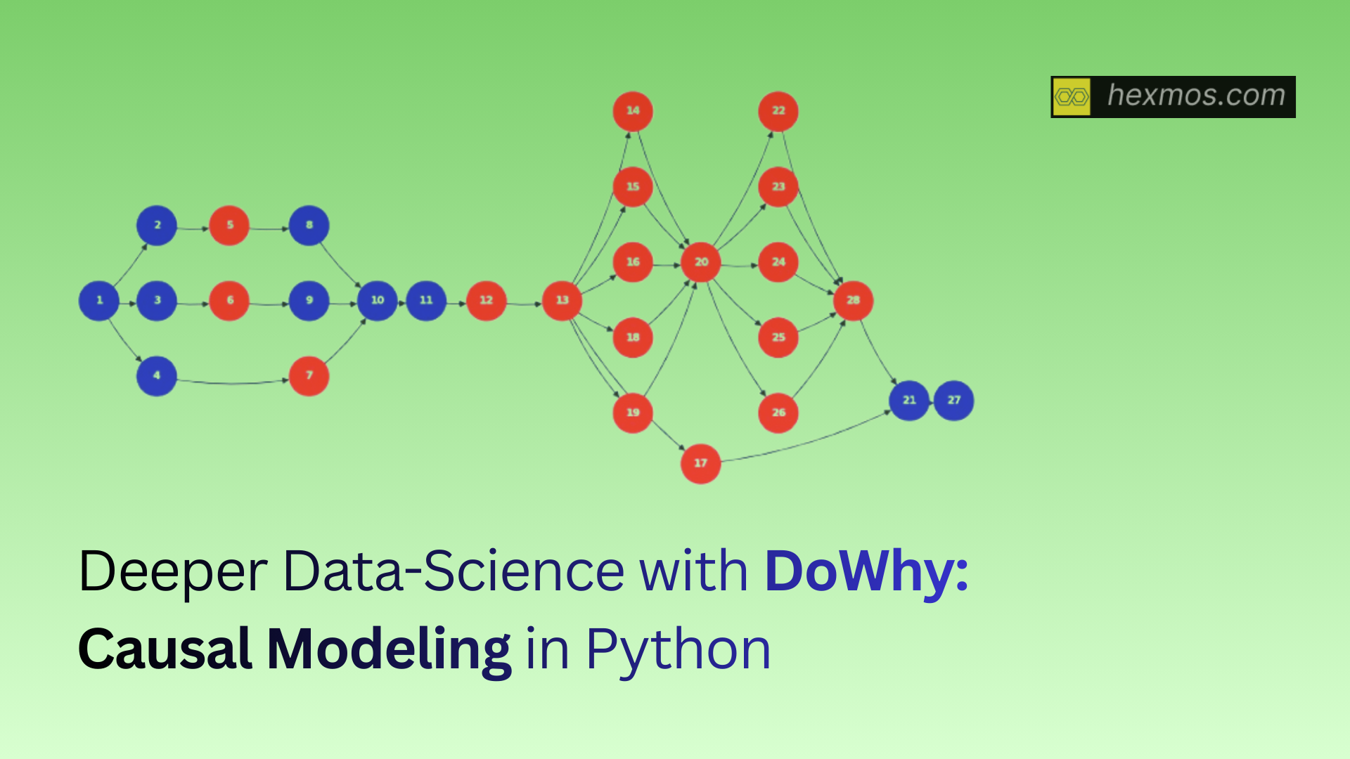
Deeper Data-Science with DoWhy: Causal Modeling in Python
Learn how causal inference with DoWhy goes beyond prediction to answer 'what if we intervene?' questions. This tutorial uses a student attendance example to demonstrate the difference between correlation and causation in data science.

Old ML was About Prediction; New AI is About Action
Old ML was about finding associations in data, and trying to make more accurate predictions.
But no matter how much data you collect - it is all history.
New things happen at a higher level - we must intervene - we must do something, with
some particular effect in mind.
Intervention requires having a causal model - an understanding of what factors lead to
what factors, which in turn lead to further factors and so on.
Judea Pearl's Ladder of Causation
The three levels of causal understanding are:
- Level 1: Seeing (association)
- Level 2: Doing (intervention)
- Level 3: Imagining (retrospection)

An Example
Consider an example, maybe more relevant for a CS teacher.
Observation (rung 1):
-> Students who attend more lectures score higher.
This is a correlation. Any standard ML model can learn this very well.
Now we ask a policy/action question (rung 2):
-> If we force students to attend more lectures, will scores improve?
From a purely correlational viewpoint, one might be tempted to say “yes.”
But that inference is unjustified.
Why? Because the original association may be driven by confounders:
- Motivation
- Prior ability
- Discipline
- Home environment
Students who attend more lectures may already be the ones inclined to do well. Forcing attendance could:
- Have little effect
- Backfire by reducing motivation
- Work for some groups and harm others
No amount of additional observational data from the same system resolves this ambiguity. You can add more features, more demographics, more regions -- and you are still estimating correlations under the same process.
I think the core point Judea Pearl makes is that more data alone cannot answer the specific contextually relevant question, “What if we intervene?”
A causal model changes the game because it:
- Explicitly represents assumptions about how variables influence one another
- Separates correlation from underlying deeper mechanisms
- Lets you simulate interventions (“force attendance”) rather than observations (“see attendance”)
In practice, this means combining:
- Data
- Domain knowledge
- Hypotheses about causal structure
- And real interventions or natural experiments
Only then can we reason about which actions are likely to work, for whom, and under what conditions.
Deep learning is compelling at rung 1.
But moving to rung 2 requires a different kind of knowledge, not just more data or larger models.
From Correlation to Causation: a Gentle Introduction Using DoWhy
Imagine you are teaching a computer science class.
You look at your data and notice something that feels obvious:
Students who attend more lectures tend to score higher on exams.
This feels intuitive.
It feels actionable.
It feels like something we should do something about.
So the natural next thought is:
If we force students to attend more lectures, their scores should improve.
This tutorial explains why that conclusion does not follow, even though the data seems to support it — and how causal inference (using DoWhy) helps us reason correctly.
The difference between observing and acting
Let’s slow down and separate two very different questions.
Observation question:
Among students who attend more lectures, do scores tend to be higher?
This is a question about patterns in the data. Machine learning is extremely good at answering this.
Action (policy) question:
If we force students to attend more lectures, will their scores improve?
This is a question about changing the world. This is not something standard ML is designed to answer.
The entire tutorial exists because these two questions are not the same.
Why the obvious conclusion may be wrong
To understand the problem, we need to think about why some students attend more lectures in the first place.
Common-sense reasons:
- They are more motivated
- They have higher prior ability
- They are more disciplined
- They have a better home environment
Now notice something important:
These same factors also affect exam scores.
So when we see:
High attendance → high score
we might actually be seeing:
High motivation → high attendance
High motivation → high score
Attendance might just be a signal, not the cause.
Confounders explained in plain language
A confounder is a variable that:
- influences the thing you want to change, and
- influences the outcome you care about
In this example:
- Motivation affects attendance
- Motivation affects score
That makes motivation a confounder.
Here is what that looks like visually.

This diagram is not something we learn from data.
It is something we assume based on domain knowledge.
This explicit statement of assumptions is the core of causal reasoning.
Why “just collecting more data” does not solve this
A very common reaction is:
“Okay, let’s collect more data and control for everything.”
But notice:
- You are still observing the same system
- Students are still selecting themselves into attendance
- Confounders still exist
More data makes correlations more precise.
It does not turn them into causal answers.
This is a key idea emphasized by Judea Pearl:
Observational data alone cannot answer interventional questions.
What causal inference adds
Causal inference does not magically extract causation from data.
Instead, it forces you to:
- State your assumptions clearly
- Check whether your question is answerable under those assumptions
- Separate what you assume from what the data says
The DoWhy library is built around enforcing this discipline.
From this point onward, we are no longer interested in prediction accuracy.
We are interested in answering a single causal question:
What happens to exam scores if we intervene and increase attendance?
Everything that follows exists only to answer this question honestly.
What is DoWhy?
DoWhy is a Python library that implements a simple rule:
Every causal analysis must go through the same four steps.
- Model: State your causal assumptions
- Identify: Check whether the causal effect can be computed
- Estimate: Compute the effect
- Refute: Stress-test the result
If you skip the first step, DoWhy will not proceed.
This is intentional.
Installing the required tools
You will need the following Python packages:
pip install dowhy statsmodels graphviz pydot pygraphviz
You also need the Graphviz system binary:
- Linux:
sudo apt install graphviz - macOS:
brew install graphviz - Windows: install from https://graphviz.org
This allows us to render causal graphs.
Defining the problem in terms friendly to code
Before writing any code, let’s name everything clearly.
| Variable name | Meaning |
|---|---|
| attendance | number of lectures attended |
| score | exam score |
| motivation | internal drive |
| ability | prior academic ability |
| discipline | study habits |
| home_env | home support environment |
These names are intentionally explicit and boring. We prefer clarity to ease understanding.
Writing down the causal assumptions explicitly
Now we translate our earlier reasoning into a formal causal graph.
Causal graph in Python (pygraphviz)
from pygraphviz import AGraph
from IPython.display import Image, display

def draw_graph(graph):
    graph.layout(prog='dot')
    display(Image(graph.draw(format='png')))

graph = AGraph(directed=True)

edges = [
    ("motivation", "attendance"),
    ("ability", "attendance"),
    ("discipline", "attendance"),
    ("home_env", "attendance"),
    ("motivation", "score"),
    ("ability", "score"),
    ("discipline", "score"),
    ("home_env", "score"),
    ("attendance", "score"),
]

graph.add_edges_from(edges)
draw_graph(graph)

This graph encodes what we believe about the world, not what the data tells us.
If these assumptions are wrong, the conclusions will be wrong -- and that is an honest failure mode.
Why we use synthetic data in this tutorial
For beginners, real-world data is confusing because:
- The true causal effect is unknown
- Many things happen at once
- It is hard to tell whether a method worked
Synthetic data solves this:
- We design the data-generating process
- We know the true causal effect
- We can check whether our method recovers it
Generating student characteristics
Each student has latent traits that influence their behavior.
import numpy as np

def generate_student_traits(num_students):
    return {
        "motivation": np.random.normal(0, 1, num_students),
        "ability": np.random.normal(0, 1, num_students),
        "discipline": np.random.normal(0, 1, num_students),
        "home_env": np.random.normal(0, 1, num_students),
    }
Think of these as underlying causes we do not control directly.
Generating attendance from traits
Attendance is not random.
It depends on student traits.
def generate_attendance(traits):
    return (
        0.8 * traits["motivation"]
        + 0.7 * traits["discipline"]
        + 0.6 * traits["ability"]
        + 0.4 * traits["home_env"]
        + np.random.normal(0, 1, len(traits["motivation"]))
    )
This reflects the real world idea that motivated, disciplined students attend more.
Generating exam scores
Scores depend on both traits and attendance.
def generate_score(traits, attendance):
    return (
        1.2 * traits["ability"]
        + 1.0 * traits["motivation"]
        + 0.8 * traits["discipline"]
        + 0.6 * traits["home_env"]
        + 0.1 * attendance  # true causal effect
        + np.random.normal(0, 1, len(attendance))
    )

Important detail:
- Attendance has a small but real causal effect
- Most of the signal comes from confounders
This is intentional.
The naive approach: regression on attendance
Most people would start with:
score ~ attendance
This answers:
Among students who attend more, do scores differ?
The answer is yes -- strongly.
But this is still an observational question.
It does not tell us what happens if we force attendance.
Building the DoWhy causal model
Now we tell DoWhy what question we want to answer and under which assumptions.
from dowhy import CausalModel
import networkx as nx

# Convert pygraphviz.AGraph to networkx.DiGraph manually
nx_graph = nx.DiGraph()
for node in graph.nodes():
    nx_graph.add_node(str(node))
for edge in graph.edges():
    source = str(edge[0])
    target = str(edge[1])
    nx_graph.add_edge(source, target)

model = CausalModel(
    data=df,
    treatment="attendance",
    outcome="score",
    graph=nx_graph
)
This is where causal inference differs from ML.
We are not asking the model to discover structure.
We are telling it what structure we assume.
Identification: checking whether the question is answerable
Before estimating anything, DoWhy asks a surprisingly strict question:
Given our assumptions and our data, is the causal question even answerable?
This step is called identification.
At a high level, identification asks:
- Are there paths that leak spurious association from attendance to score?
- Do we observe enough variables to block those paths?
In causal language, these unwanted paths are called backdoor paths.
What is a backdoor path (intuitively)?
A backdoor path is any way information can flow from attendance to score without actually going through attendance.
For example:
attendance ← motivation → score
This path creates correlation, even if attendance itself has no effect.
To block this path, we must condition on motivation.
What DoWhy does during identification
When we run:
estimand = model.identify_effect()
print(estimand)
We get:
Estimand type: EstimandType.NONPARAMETRIC_ATE

### Estimand : 1
Estimand name: backdoor
Estimand expression:
      d
─────────────(E[score|motivation,ability,discipline,homeₑₙᵥ])
d[attendance]
Estimand assumption 1, Unconfoundedness: If U→{attendance} and U→score then P(score|attendance,motivation,ability,discipline,home_env,U) = P(score|attendance,motivation,ability,discipline,home_env)

### Estimand : 2
Estimand name: iv
No such variable(s) found!

### Estimand : 3
Estimand name: frontdoor
No such variable(s) found!

### Estimand : 4
Estimand name: general_adjustment
Estimand expression:
      d
─────────────(E[score|motivation,ability,discipline,homeₑₙᵥ])
d[attendance]
Estimand assumption 1, Unconfoundedness: If U→{attendance} and U→score then P(score|attendance,motivation,ability,discipline,home_env,U) = P(score|attendance,motivation,ability,discipline,home_env)
DoWhy inspects the causal graph and concludes:
- There are confounding paths
- All of them go through:
- motivation
- ability
- discipline
- home_env
- We observe all of these variables
Therefore:
If we adjust for these variables, the causal effect of attendance is identifiable.
This is what the output is telling us, in mathematical language.
When you see:
E[score | motivation, ability, discipline, home_env]
you should read it as:
"Compare students who are similar in motivation, ability, discipline, and home environment -- and differ only in attendance."
This is the core causal idea.
This step asks:
- Are all confounding paths blocked?
- Do we observe the variables we need?
If the answer is no, DoWhy stops.
Estimation: approximating an intervention using data
Now that DoWhy has confirmed the causal effect is identifiable, we can estimate it.
We run:
estimate = model.estimate_effect(
    estimand,
    method_name="backdoor.linear_regression"
)
print(estimate.value)
We get:
0.0927561466288897
This answers the real question:
If we intervene and increase attendance, how much does score change?
This is mathematically different from correlation.
This number answers exactly one question:
If we intervene and increase attendance by one unit,
how much does the expected exam score change?
It does not mean:
- “Students who attend more score higher”
- "Attendance is a strong predictor"
- “Attendance explains most variance in scores”
Those are observational statements.
This number is an interventional effect.
Why this number is so much smaller than the correlation
Earlier, the naive regression showed something like:
attendance coefficient ≈ 0.98
attendance coefficient ≈ 0.98
That number mixes together:
- the true causal effect of attendance
- the effect of motivation
- the effect of ability
- the effect of discipline
- the effect of home environment
Once we explicitly adjust for those confounders, only the direct causal effect remains.
That direct effect is small — by construction.
This is the “aha” moment.
The “aha” result
The causal estimate tells us:
Forcing students to attend more lectures has only a small effect on scores.
This does not mean:
- Lectures are useless
- Attendance does not matter
- Teachers do not matter
It means something subtler:
Much of the advantage seen among high-attendance students
comes from who they are, not from attendance itself.
This explains why policies like mandatory attendance often:
- fail to produce large gains
- work only for specific subgroups
- sometimes backfire by reducing motivation
Causal inference does not tell us what to do -- but it tells us what will not work as expected.
Refutation: stress-testing the causal claim
After estimating a causal effect, DoWhy encourages skepticism.
The question now becomes:
Could this effect be an artifact of chance, noise, or modeling quirks?
This is the purpose of refutation tests.
Refutation does not prove the result is correct.
It checks whether the result is fragile.
Adding a random confounder
One simple refutation test is:
What happens if we add a completely random variable
and pretend it is a confounder?
If the causal estimate changes dramatically, the result is unstable.
We run:
refutation = model.refute_estimate(
    estimand,
    estimate,
    method_name="random_common_cause"
)
print(refutation)
Typical output looks like:
Estimated effect: 0.0927
New effect:       0.0928
p-value:          0.84
How to read this result
This tells us:
- Adding a fake confounder does not change the estimate
- The causal effect is not sensitive to random noise
- The result is reasonably stable
This increases our confidence -- not certainty, but confidence.
Causal inference is about disciplined doubt, not blind belief.
What this example actually teaches
This example is deliberately simple, but the lesson is deep.
You learned that:
- Prediction answers: What tends to happen?
- Causation answers: What will happen if we act?
You learned that:
- Correlation can be large
- Causal effects can be small
- Both can be true at the same time
You learned why:
- More data is not enough
- Better models are not enough
- Explicit assumptions are unavoidable
Most importantly, you learned that:
Every action embeds a causal theory, whether we admit it or not.
DoWhy simply forces us to make that theory explicit -- and then checks whether the data can support it.
Try It Yourself
Find the full example in the Google Colab